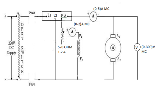
To predetermine the efficiency of a DC shunt motor at any load using Swinburne's test (no-load test method).

Introduction

Swinburne's test is an indirect method of testing DC shunt motors. It requires only a no-load test to determine the efficiency at any load. This method is economical and convenient as it doesn't require actual loading of the motor.

Principle

The test is based on the assumption that for a DC shunt motor, the flux remains constant (since field current is constant), and the losses can be divided into:

• Constant losses: Iron losses and mechanical losses (friction + windage)
• Variable losses: Copper losses (I²R losses)

Key Formulas

Advantages

• Very economical - requires only no-load test
• No need for actual loading arrangement
• Quick and convenient method
• Suitable for shunt motors where flux is constant

Disadvantages

• Not suitable for series motors (flux varies with load)
• Assumes constant flux, which may not be true due to armature reaction
• Does not account for stray load losses
• Accuracy depends on accurate measurement of armature resistance

Apparatus Required

• DC Shunt Motor
• DC Supply (Variable)
• Field Rheostat
• Voltmeter, Ammeter
• Multimeter (for resistance measurement)
• Connecting wires

Circuit Diagram

Steps

1. Measurement of Armature Resistance:
   • Disconnect the motor from supply
   • Using multimeter, measure armature resistance (R_a)
   • Note: Apply low current to avoid heating effects
   • Record the value: R_a = _____ O
2. No-Load Test:
   • Connect the motor as per circuit diagram
   • Keep the field rheostat at minimum resistance
   • Start the motor with rated voltage applied
   • Run the motor at no-load (without any mechanical load)
   • Adjust field rheostat to get rated speed
   • Note down:
     • Supply voltage (V₀)
     • No-load current (I₀)
     • Field current (I_f)
     • Speed (N₀)
3. Calculations:
   • Calculate no-load input power: P₀ = V₀ ×  I₀
   • Calculate constant losses: P_c ≈ P₀
   • For different load currents, calculate:
     • Input power: P_in = V ×  I_a
     • Copper loss: P_cu = I_a²R_a
     • Total losses: P_loss = P_c + P_cu
     • Output power: P_out = P_in - P_loss
     • Efficiency: η = (P_out / P_in) ×  100%
4. Results:
   • Tabulate the results for different loads
   • Plot efficiency vs. load current curve
   • Determine maximum efficiency point

Precautions

• Ensure motor runs at no-load (free rotation)
• Apply rated voltage only
• Measure armature resistance accurately
• Allow motor to reach steady state before taking readings
• This method is valid only for shunt motors

Given Data

No-Load Test Reading

Calculations

Efficiency Calculation at Load Current I_a = 8 A

Expected Results

• Constant losses remain approximately constant at all loads
• Efficiency increases with load up to a certain point, then decreases
• Maximum efficiency occurs when constant losses = variable losses
• For the given example: Maximum efficiency occurs when I_a²R_a = P_c